This is a very basic introduction to VMD.
So, what is VMD? In the words of its developers:
VMD (Visual Molecular Dynamics) is a molecular visualization and analysis program designed for biological systems such as proteins, nucleic acids, lipid bilayer assemblies, etc.
It is developed by the Theoretical and Computational Biophysics Group at the University of Illinois at Urbana-Champaign. Among molecular graphics programs, VMD is unique in its ability to efficiently operate on multi-gigabyte molecular dynamics trajectories, its interoperability with a large number of molecular dynamics simulation packages, and its integration of structure and sequence information.
The aim of this tutorial is to very quickly get you familiar enough with VMD to be able to view individual protein structures and the sorts of trajectories containing many structures that are produced by molecular dynamics and other simulation techniques. This document is deliberately designed to cover only the most basic features of VMD. Excellent tutorials teaching the full range of the functionality provided by the program can be found at the VMD website, here.
VMD specializes in the visualization of data from molecular simulations. In addition to PDBs several other formats are widely used to describe molecular systems. In this tutorial we focus on those associated with simulations using the CHARMM forcefield.
A PSF, protein structure file, contains all of the molecule-specific information necessary to describe a particular molecular system using the CHARMM force field. Contains information about the atom types, residues, covalent bonds, and selections of atoms used to determine force terms in molecular dynamics or Monte Carlo simulations (such as angle and dihedral terms) but NOT coordinates.
A PDB file contains atomic coordinates and type alongside information about how they are organized into residues. For non-standard residues connectivity can be specified using CONECT records, however VMD ignores these and if no PSF is provided explicitly defining connectivity bonds are assigned using a distance cut off. PDB files may contain multiple sets of coordinates for the same system.
DCDs contain ONLY coordinates and no information about atoms or their connectivity. They are binary files and consequently much more efficient than PDBs for storing large numbers of coordinate sets. DCD files must be used in conjunction with a structure file.
This tutorial assumes:
To start the program:
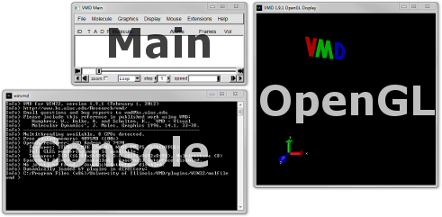
Upon opening VMD opens three windows (Figure 1): the Main, OpenGL Display and Console (or Terminal on OS X) windows. To end a VMD session, go to the Main window, and choose File -> Quit. You can also quit VMD by closing the Console or Main window.
In this section we will load a single structure from a PDB and learn how to view it from different angles and to alter the way it is rendered on screen.
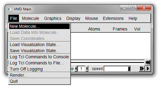
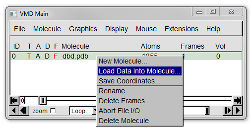
From the menubar in the Main window select File -> New Molecule... (Figure 2).
A Molecule File Browser window similar to that shown in Figure 3 should now open. Select the Browse.. button (circled in red in Figure 3). This will open a file selection dialog. Navigate to the PDB file, dbd.pdb, which you downloaded earlier, select it and click Open.
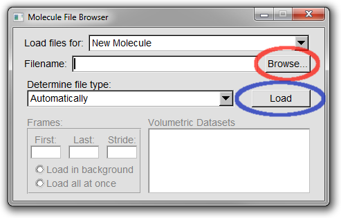
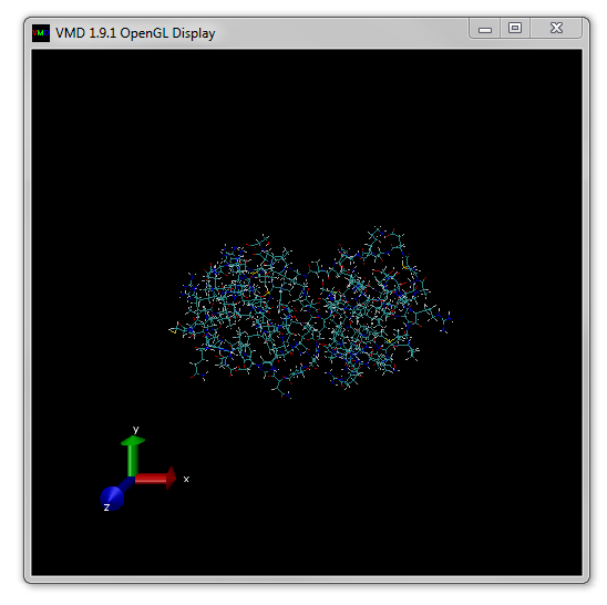
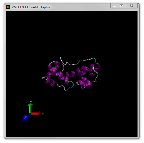
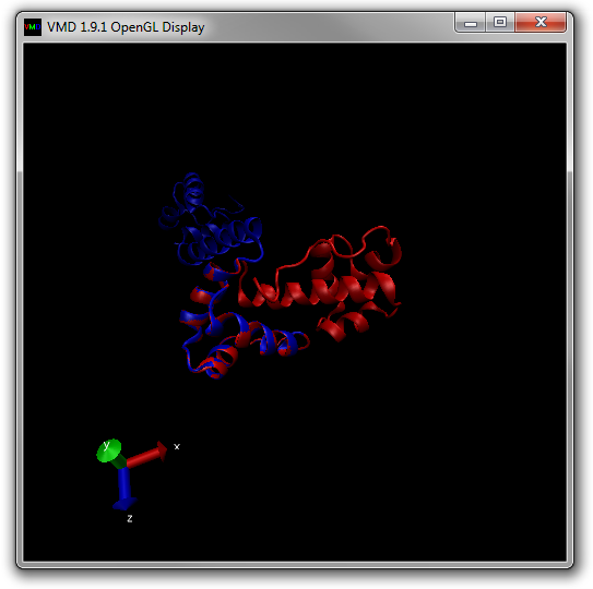
You should now have been returned to the Molecule File Browser window (the structure will not yet have been loaded). To load the file you need to click the Load button (circled in blue in Figure 3). The structure should now be loaded and the OpenGL Display window look something like Figure 4.
Notice that once the molecule is loaded basic information including the name of the file and number of atoms appear in the Main window.
Once the structure is loaded you can close the Molecule File Browser at any time.
From the menubar in the Main window select Mouse (Figure 5).
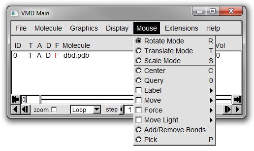
A larger array of options for how the mouse interacts with the molecule shown in the OpenGL Display. We will concentrate on the first four options: rotate mode, translate mode, scale mode and center. The keyboard shortcut for each option is shown next to the choice in the menu (for example pressing 't' when the OpenGL windows is selected will change into translate mode). By default VMD uses the rotate mode.
Generally, to change the viewpoint you need select the OpenGL Display windows, hold the left mouse button and move the mouse (the right mouse button can be used in rotate mode, see below). Have a play with all of the modes below until you feel comfortable changing the view and switching between the various modes. You can easily tell which mode you are in because each one has a distinctive cursor (Figure 6).
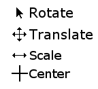
Rotate mode: With the left mouse button held moving the mouse horizontally rotates the molecule around the vertical axis, up and down around a horizontal one. When the right mouse button is held then the rotation is performed around an axis running into and out of (i.e. perpendicular to) the screen.
Translate mode: When you hold down the left mouse button you can now move the molecule up, down, left or right in the viewing plane.
Scale mode: Moving the mouse left or right whilst holding the left mouse button zooms in and out.
Center: The centre option is not a direct method for altering the view point. It is used to pick a point about which to perform a rotation. Once you have selected a center point change to Rotate mode to perform the rotation.
At any point you can reset the view by pressing '=' whilst the OpenGL Display is selected (you can also use the menu option Display -> Reset View.
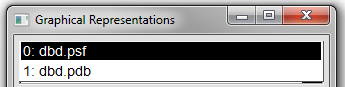
Select Graphics -> Representations... from the menubar of the Main window. A new Graphical Representations window will open looking like Figure 7. Section Figure 7 (a) shows the current representation being highlighted. It shows the style of the representation (in this case Lines), the colouring method (Name) and the selection of atoms to which this representation is applied. The selection is determined by the contents of the input box shown in Figure 7 (b). The current selection is for all atoms. The language used to select atoms in VMD is documented in the section of the user guide here.
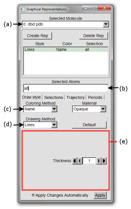
Try changing the Coloring Method by choosing different options from the drop down menu shown as Figure 7 (c).
When dealing with simulations multiple structures are commonly saved together in files called 'trajectories'. An example of a trajectory format is DCD (used by NAMD and CHARMM). Such files contain only coordinates and no information about which atoms are represented. In order to vizualize the atomic structure represented by a trajectory it has to be combined with a file containing structural information. PDB files contain both structural and coordinate information and can perform this role, other filetypes such as PSF files contain only structural information and no coordinates.
The trajectory from this point assumes that you have already loaded the dbd.pdb PDB files into VMD. If that is not the case go through the instructions for [Loading a Molecule].
In the Main window either select File -> Load Data into Molecule... or right click on the line for dbd.pdb and select Load Data into Molecule... from the menu (see Figure 9a below).
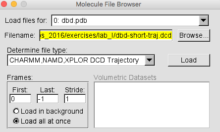
Like when we loaded a PDB previously a Molecule File Browser window should appear. Browse to the dbd-short-traj.dcd and Load it.
As the trajectory loads you will see the number of frames increase in the Main windows and the structure in the OpenGL Display update.
If you are loading a DCD file with a large number of trajectories, it will load faster if you choose the Load all at once option in the Molecule File Browser as shown in Figure 9b below.
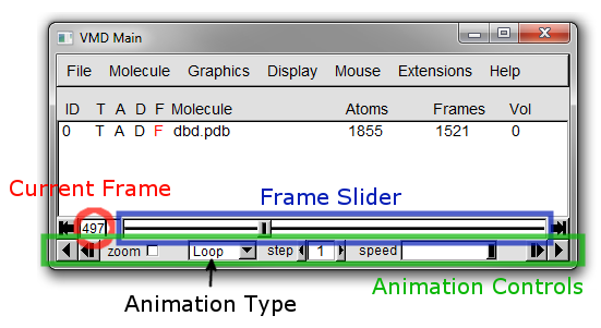
The Main window should now look something like it does in Figure 10 below, where the current frame is circled in red.
Note that frames are counted from zero in VMD. In this case, frame zero is the structure loaded from the PDB. However, if you load a structure information only file, such as a PSF, instead of a PDB, then frame zero will be the first frame of the DCD.
You can use the slider highlighted in blue in Figure 10 to move to any frame you desire. It is also possible to type in a specific frame number in the current frame region.
Beneath these controls are the animation controls (highlighted in green in Figure 10). These allow you to play through the frames of the trajectory. Forwards and backwards play buttons can be found at either end of the controls. Between these are controls which alter the way the animation plays. The 'step' controls the gap between the frames which are displayed and 'speed' is self explanitory. The animation type drop down menu controls what happens when the animation has played the last frame in the current direction:
Once: The animation terminates.
Loop: The animation plays again from the start (opposite end).
Rock: The animation reverses direction.
Play with these controls until you are happy you understand how they work.
This tutorial describes how to load and visualize simulation topology and trajectory files in VMD.
Files needed for this tutorial (located in the $HOME/Desktop/aps_2016/exercises/lab_I directory):
In this section we will load coordinates into two molecules. The first will contain a trajectory obtained from a Monte Carlo simulation and the second the PDB structure used to start that simulation.
This time we will load the trajectory using the structure information in the PSF file.
Start a new VMD session.
From the menubar in the Main window select File -> New Molecule... .
From the Molecule File Browser window Browse to the dbd.psf. The file type should be automatically detected as 'CHARMM, NAMD, XPLOR PSF'.
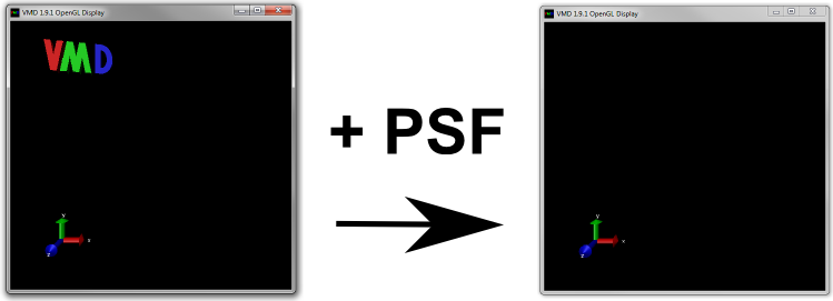
Click Load. No molecule will appear in the OpenGL display but the VMD logo should disappear as shown in Figure 11 below. The Structural connectivity information has been loaded without any coordinates.
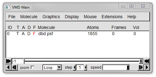
In the Main window you should see an entry with an ID of 0 and a Molecule name of dbd.psf with 1855 atoms, but 0 frames, as shown in Figure 12a below.
Now we need to load coordinates into our molecule from a DCD. Right click on the line for dbd.psf and select Load Data into Molecule... from the menu. Just as for the PSF a Molecule File Browser window should appear. Browse to the dbd-short-traj.dcd and Load it.
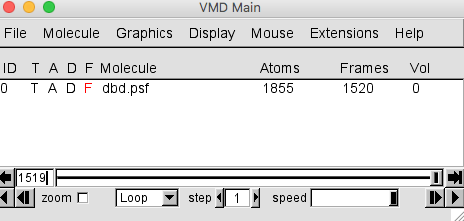
Now a structure should be visible in the OpenGL display and now the dbd.psf ID 0 entry should have 1520 frames as shown in Figure 12b below.
Since we loaded a structure information only PSF file in this case, frame zero is the first frame of the DCD.
From the menubar in the Main window select File -> New Molecule... .
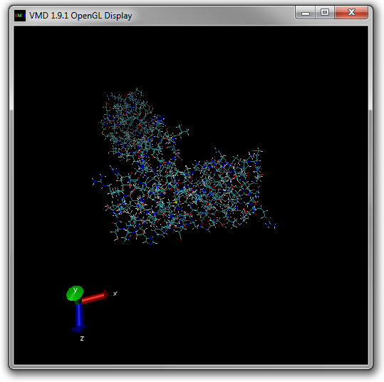
From the Molecule File Browser window Browse to the dbd.pdb file you downloaded earlier. The file type should be automatically detected as 'PDB'. The OpenGL window should now look like Figure 13 below.
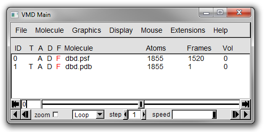
There should now be entries for two molecules (ID 0 for dbd.psf and 1 for dbd.pdb) in the Main window (see Figure 14 below). Both should have the same number of atoms but differ in the number of frames.
Select Graphics -> Representations... from the menubar of the Main window.
A new Graphical Representations window will open.
Set the following settings:
One of the molecules (1: dbd.pdb) should have changed appearance to a cartoon in the OpenGL window.
Switch molecules by clicking on the down arrow at the end of the Selected Molecule box and choosing '0: dbd.psf' from the menu list that appears (see Figure 15 below).
Alter the Coloring Method and Drawing Method to the same setting as the previous molecule.
Your OpenGL window should now look like Figure 16 below.
Try to animate the trajectory by moving the Frame Slider at the bottom of the Main window. You should not be able to change the visualization. In the next section we will see why not and right this terrible injustice.
In Figure 17 below, three columns in the Main window information panel are highlighted. These columns provide toggles for the various statuses that can be assigned to molecules.
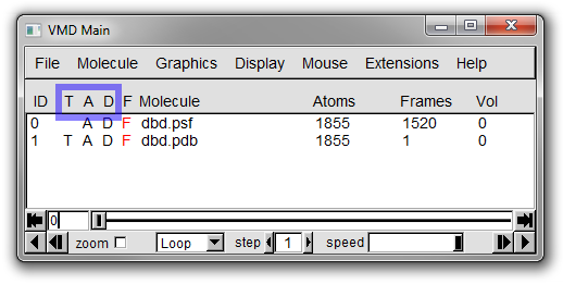
The three letters each indicate a different status setting for each molecule:
(T)op molecule - indicates the default molecule for all actions (only one moelcule can have this status)
(A)ctive - if set the trajectory of the molecule will be updated in any animation
(D)rawn - indicates if the molecule is being displayed in the OpenGL window
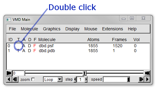
The reason that we cannot animate our trajectory is that molecule 1 (dbd.pdb) has the (T)op status and has only one frame. To change the top molecule double click on the T column region of molecule 0 (dbd.psf), the location to click is shown in Figure 18 below.
Now try to animate the trajectory by moving the Frame Slider at the bottom of the Main window. You should now see the variation over the trajectory compared to the static PDB.
Try toggling the (D)rawn status of different molecules.
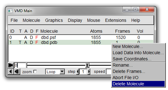
To delete a molecule right click on it on it in the Main window and select Delete Molecule (see Figure 19 below).
This tutorial describes basic scripting in VMD. Anything that can be done in the graphical interface can also be done with text commands. Knowledge of some basic text commands is useful for structure building and MD.
Files needed for this tutorial (located in the $HOME/Desktop/aps_2016/exercises/lab_I directory):
This section discusses the basics of the Tcl scripting interface in VMD. More information on how to use scripting in VMD can be found in the User Guide. More information on the Tcl language as well as the Tk extension for graphical user interfaces can be found here.
To execute Tcl commands, you can use the TkConsole window or the VMD console window, which is the terminal window that opens up when you start VMD. Here we will use the TkConsole window.
Let's load a molecule using text commands.
In the TkConsole window:
Navigate to the $HOME/Desktop/aps_2016/exercises/lab_I directory using standard OS commands as shown in Figure 19 below.
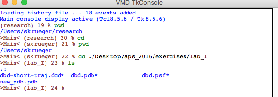
Type mol new dbd.pdb. The Main window should show that a molecule is now loaded and it should be visible in the OpenGL window. The VMD console window (that opened when you started VMD) will show the statistics for the molecule that we just opened.
To operate on a molecule or part of a molecule, the first command that must be executed is the atomselect command.
In the TkConsole window:
Type set sel [atomselect top "all"].
This creates a selection, sel, that contains all the atoms in the molecule and assigns it to the variable sel. Instead of a molecule ID (which is a number), we have used the shortcut “top” to refer to the top molecule. The result of atomselect is a function. Thus, $sel is now a function that performs actions on the contents of the “all” selection. If the command was typed correctly, you should see a reply such as atomselect 0, as shown in Figure 20 below.

Now, let's operate on the atom selection that we have defined.
Type $sel num.
This returns the number of atoms in the molecule. Don't forget the $ sign in front of sel. This should return the same number of atoms that is shown in the Main window.
Let's try making some measurements.
Type:
The two commands, move and moveby can be used to move the molecule on the screen and change its coordinates (as opposed to rotating or translating the molecule with the mouse, which only changes the view and not the coordinates).
Type:
The “B” field of a PDB file typicallystores the “temperature factor” for a crystal structure and is read into VMD’s “Beta” field. We can make use of this field to store our own numerical values. VMD has a “Beta” coloring method, which colors atoms according to their B-factors. By replacing the Beta values for various atoms, you can control the color in which they are drawn. This is very useful when you want to show a property of the system that you have computed. You can obtain and set many atomic properties using atom selections, including segment, chain, residue, atom name, position (x, y and z), charge, mass, occupancy and radius, just to name a few.
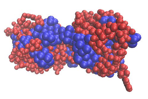
Let's use the "Beta" field to identify the hydrophobic residues in our molecule. First, set the Coloring Method to Beta and the Drawing Method to VDW using the Graphical Representations window. All the residues should be the same color since we haven't identified the hydrophobic residues yet.
In the TkConsole window:
Now, let's make the hydrophobic residues stand out.
Your molecule should now look something like the one in Figure 21 below.
VMD is not only a molecular viewer but also allows you to analyse structures and trajectories, convert file format, render graphics for publication and many more things well beyond the scope of this tutorial. When you want to try out these features best place to start is the User Guide.
When you, inevtiably, run into difficulties a good first port of call is the mailing list.